Image sensors: Analysis preparation

Image sensors: Noise analysis preparation

You can read a lot on image sensor analysis theory, but there isn't much written on practice. This page is about moving from theory to craftsmanship.

Does everything work fine?

Images, in the context of sensor analysis, are the closest possible mapping of photons to bits possible.

Raw images offer that with one exception: No photons should cause the pixel value 0 aka black. That's not how image sensors work, but for analysis, the black level offset (sometimes called bias) should be 0. So some raw image conversion is required to subtract the global black level offset. In case the sensor provides masked pixels for offline pixel offset correction, that's fine as well.

In case you cannot get raw images, you may have to choose a special image file format, because almost all image formats use gamma encoded (or similar) brightness. Sometimes an option is available to violate that requirement and store linear brightness in an image format that requires gamma encoded brightness.

Once enabled, the linearity is rarely a problem, except when pixel values are clipped: Cutting off noise instead of letting pixels have negative values means to lift the average of black pixels artificially. That can be avoided by using the FITS image format, which allows negative values. If your tools do not allow to use FITS, you'll have to live with a slight non-linearity. Cutting off noise above the full well capacity lowers the average of almost fully exposed pixels. File formats don't rescue you there: Avoid getting near exposure limits.

Does the camera have bugs? A poor shutter may lead to more exposure for the first image of a series or introduce a gradient. Firmware bugs could cause bad images, e.g. when switching exposures. There could be broken images at high frame rates. The exposure control may not be as accurate as it promises. Perhaps the brightness just jumps around a little bit.

I have personally seen all of these. For that reason, it makes sense to check if the camera works fine to be sure subsequent analysis yields correct results.

Suitable illumination for noise analysis

Ideally, mount the camera without optics at an integrating sphere, which provides a field of light that is homogeneous in both light density and ray angle distribution. The latter avoids many optical problems, e.g. dust, which causes small dark spots and diffraction patterns. This is an example of an image taken with collimated light, which shows all of these. This is the same sensor with the same dust particles as below! If you see such patterns, the illumination is not suitable for pixel analysis.

Stretching this image shows the mixture of noise and dust very well. The different noise structure is caused by a different exposure time than the image below. Trying a noise analysis with such images would be hopeless.

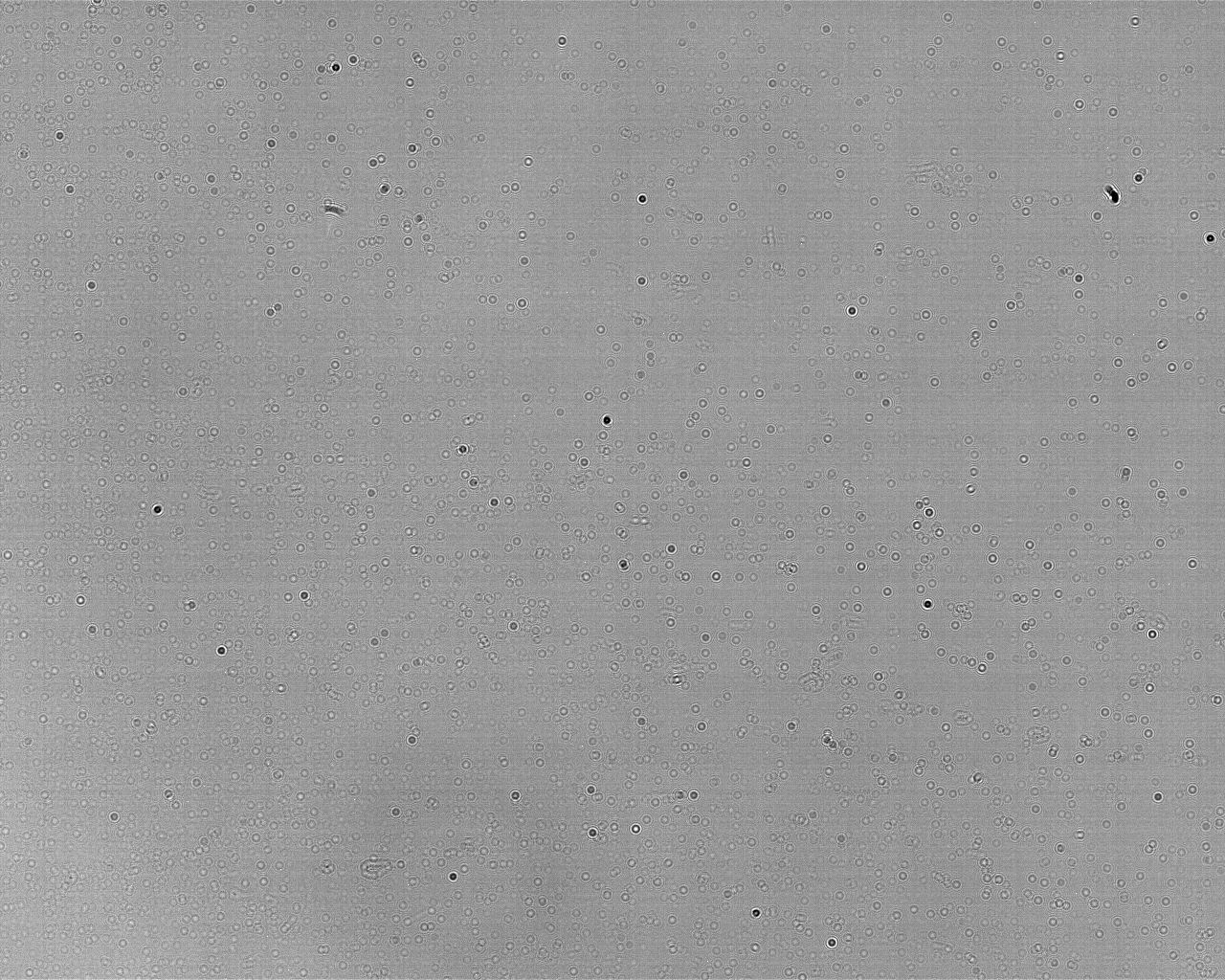
Since photon noise is not linear, but squared to the brightness, it disturbs averaging the noise. If you subtract two images of equal brightness, only noise is visible, but the diffraction of dust shapes the noise, so it remains visible. Yes, dust can ruin noise analysis.

Using a lens to image a white wall, even if defocused, cannot be recommended: The light ray angle likely varies for different pixels and it is very easy to end up with a different amount of light per pixel (vignetting).

Yet, too wide angles may be bad as well, because they may lead to light travelling in unexpected ways through microlenses, showing reflections that are not or much less visible with focused light. In that way, some distance from the integrating sphere port will restrict the angle and still provide the homogeneous field, but also show dust a little more.

Relation of exposure time and brightness

Once the illumination of the image is ok, acquire multiple images with different and possibly random exposure times, best small bursts of each time. That verifies both burst shots as well as switching exposure times wildly. The brightness should cover typical exposure times at base gain/ISO. For reproducibility, measure the brightness with a Lux meter (green light preferred) or photo sensor (select correct wavelength of monochromatic light for correct results).

Inspect some images visually. They should be of uniform brightness. This is an example of the MT9M001 sensor in a QHY5 compatible camera with 570 nm at 0.18 μW/cm² using the 8 MSB (click for full resolution).

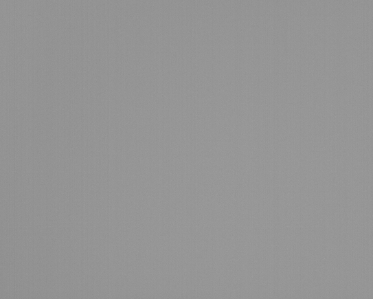
Stretching the contrast with image processing shows the noise. This image shows some banding noise (row and column pattern) as well as unstructured noise. There are no spots or shapes.

The histogram should be narrow and shaped as gauss curve. That shows you are dealing with regular, expected noise only.

Finally compute the average brightness and the standard deviation of row and column averages. The absolute value of the standard deviation does not matter, but unexpected changes will detect oddities, like gradients. This diagram is fine: The error bars are narrow, the black level is at 0, everything is continuous and the slight non-linearities at the low and high end are common.

This step often takes most of the time and yields surprises in either the camera, the software or the setup. I highly recommend not to skip it.

Do not believe in what you see

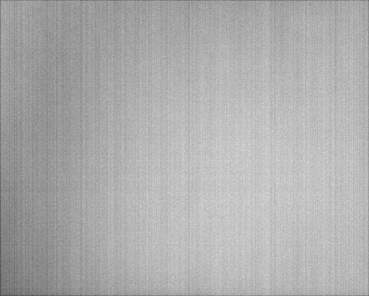
This is an example of a gradient that occurs for exposures larger than 220 ms with a buggy QHY5 firmware. The gradient is a few percent, but human vision cannot see small differences in brightness, especially if there is no sharp edge:

Stretching the contrast shows clearly that the image is dark at the top and bright at the bottom, though:

Do not rely on human vision to evaluate image sensors. Now that you know what to look for, you can probably see the gradient in the original image, too. The jumping standard deviation indicated that something went wrong:

This would have been missed without thorough preparation and visual inspection only. Astrophotography often multiplies the brightness and it can be very confusing if a gradient appears to origin out of nowhere.